- You are here:
-
Home

-
Articles
-
Perception
-
ROOT
- Articles
Articles
Perception
Written by Pavol Durisek- Details
-
Category: Articles
-
Published: 19 June 2018
-
Hits: 6864
(very early draft)
Introduction
From 60s to 80s a huge effort was being made to develop a computer vision system. Despite early enthusiasm only one solution was giving some significant and practical results to solve this problem in general, the neural networks which now is just re-branded as deep neural networks. After that, the search for understanding visual perception slowed rapidly down. Although developing artificial intelligence shared similar experience, its development is still active and new ideas seems to occasionally appear.
There are many views and believes about the theory of intelligence and for some time now there have been an effort to build one. We also know that it can be done because we already have one (in a biological world) but we don’t know how to build it or if we are able to build it. It is said that intelligence is a universal tool to solve difficult problems and also that it tries to find an optimal solution for a problem. It is our general view but is it really the case? Its seems to me to be a similar misconception as when we try to test computers on human intelligence by giving them task that are difficult for us, like solving mathematical problems, playing chess or computer games or composing music. We do test humans on those because they are difficult for us. If we want to test how computers are human alike we should test them by giving them tasks that are easy to us, so easy we don't even notice, like task from (visual) perception, yet still unchallenged by today's computer.
Before we deep into the theory of intelligence and perception in particular let's have a thought why they exists and what is they purpose by examining living organisms which posses those.
What is it that all known currently living organism share and all have in common? It is they presence. If we assume that all living things are driven by evolutionary processes then it means that from this point of view (almost) all the properties they have will support this basic one - the ability to survive (either by adapting or changing their environment).
So from now on we can consider intelligence as a tool with one purpose only – to help to survive (in terms of species, not necessarily individuals, evolution would disregard any other purpose). But it is not the only tool nor strategy to do so, all others co-existing on the same time and same environment, are equally good. One could say that e.g. playing the piano is just a random action and nothing to do with survival. Human lives in environment that have not just physical properties, but also a complex social one. So the question rather would be, why complex social interactions emerged and why it is so important for survival? Maybe the answer lays in the work of Danny Hillis on co-evolution1. Perhaps it is a strategy to avoid evolutionary decline of a species.
Now let’s think about how intelligence help to survive. While non-living things are subject to change from the environment, living things can intervene this process and act on this change in order to survive. Basic adaptation does not need a complicated control mechanism, more sophisticated requires more advance techniques, like identification of the situation and an adequate response. While less intelligence creatures could try to survive by outnumbering and randomly modifying itself (so some of them would meet required fitness), more intelligent organism could do the exact thing with much less number.
It appears that intelligence and perception as a part of it is an important tool to go from a more statistical survival to a more intentional survival.
How perception might work? Identifying the situation and pairing with the right action improves survivability. And those are inseparable. From an evolutionary point of view this means that this is not about as realistically and objectively describing the surrounding environment as possible, but extracting and interpreting those information from the input in the way which would help trigger successful actions in terms of survivability for the given organism. This is not independent from the organism and its surrounding. So, to me, intelligence is a successful pairing of a perception to an action. Solving problems are not different. Here, perception is identifying the problem and action means finding a solution for it. Perception is not just understanding the surroundings, but also understanding internal state of the organism, or internal state of the processes involved in intelligent behavior. As we can see perception is one of the key to intelligent behavior.
Also need to mention that back in time when computers were developed John Von Neumann and his team was coping with a problem to build a reliable machine from very unreliable parts, what evolution did was building a powerful and efficient system using very slow and relatively energy consuming parts.
Visual perception
In most biological systems, emitted or reflected light enters trough the lens into the retina where it is detected by photosensitive cells and transformed into neural signals in order to understand surroundings. So, why is this so challenging? One of the problem is the ambiguity between sources of retinal stimulation and the retinal images that are caused by those sources. This problem is often called inverse problem in optics when the exact same image in the retina could be created by an infinite number of object of different size, orientation and distance. We need to also consider combinations of source of light, reflection and absorption of the object and absorption of the environment between the object and the observer. And even a simple fact, that the photo-receptor generates the same neural signal for a number of combination of wavelength (color) and intensity. However, perception does not have to try to be as objective and realistic as possible - that is not its purpose - but trying to be as helpful as possible in the process of survival. The success of perception will be determined by a success of an action that came out as a result of this percept.

Figure 1 The squares marked A and B are the same shade of gray, yet the brain can (correctly) distinguish between them by understanding the whole scene based on past experiences
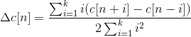
Another problem is how to effectively extract and interpret meaningful information from the vast amount of data entering the system in a robust way and a reasonable time.
The simplest possible visual information is an image uniformly composed of the same color and brightness. There is no need to send and process data from every photo-receptor separately but just from one of them. Also this information has low value and reliability. When the input image become more complex, what is enough to send to the system are just changes in color and brightness in space (gradients/edges) and time (movements). It is not just to reduce data but also to reduce some ambiguity. While a constant color or intensity significantly change if light conditions changes; changes on gradients remain under more broader change of light conditions (see Figure 1 - squares A and B are exactly the same shade of gray due those light conditions so indistinguishable by computers, edges defining those squares however are clearly detectable). Those individual edge points can be further hierarchically grouped to more complex structures and non relevant data can be further reduced (e.g. changing absolute position to relative one, adding position, scale, rotation invariance, or even more generalizing the object etc.).
In biological systems on and off center cells are used to detect these gradients. In computer vision Difference of Gaussian or Laplacian of Gaussian are commonly used for the same purpose. Do detect gradients from a broad range of magnitude (slope of change, not orientation) usually these filters are applied on each level of the pyramidal representation of an image. To reduce the amount of calculation I would suggest to use LoG filters of the same size, but with different sparsity and increase sparseness just when and where edge is not detected (avoiding computation redundancy). While often is mentioned that Gabor filters more resemble biological visual processing at early stages, they are much more computational costly without significant advantages (orientation of gradients we can get in different computationally more plausible way).
Computer Vision has also a very elegant algorithm called Hough Transform which is relevant to the Radon transform and is used to detect geometric features like straight lines, circles, ellipses that can be described either analytically or in case of Generalized Hough transform, it can detect an arbitrary shape described by its model. The main disadvantage is it speed.
Hough Transform
Let's have a look at a simple line detector. In image space the lines are described by an equation:

, or to also include vertical lines, by equation:


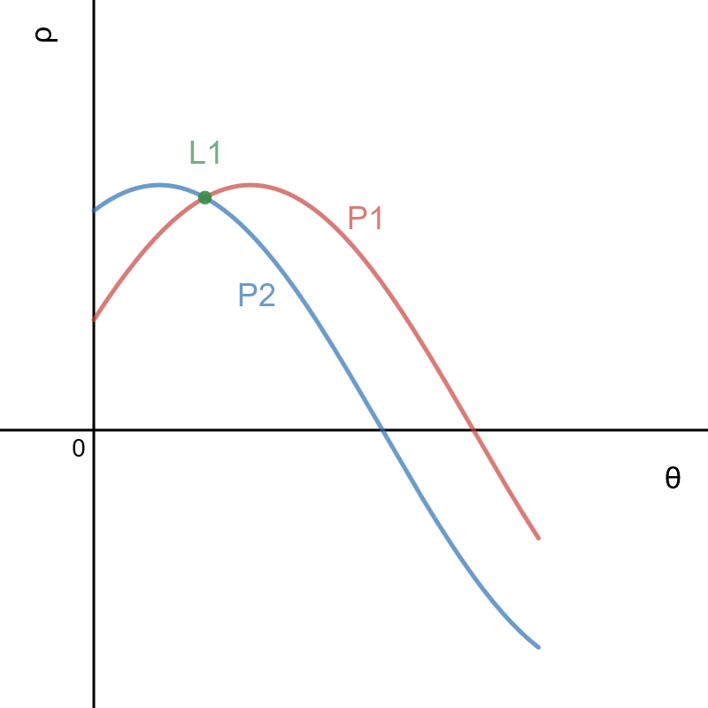
Figure 2.a, 2.b Points P1, P2 and Line L1 in image space (left) and parameter (Hough) space (right)
Every single point in image space is represented by a unique sinusoid in parameter (Hough) space, which represent a set of lines that crosses that point. In other hand, every point in Hough space represents a whole line in image space. A set of two or more points that form a straight line will produce sinusoids which cross at the (ρ, θ) for that line.
In general we can use different equations with different parameters to detect different features. Also adding additional parameter we can achieve e.g. size or orientation invariance but it will cost performance. I believe the same can be achieved also differently without loosing performance.
To avoid repeated calculations, most of Hough transform implementations pre-calculates values of sin(θ) and cos(θ) and reused them from a look-up table.
Randomized Hough Transform
It takes advantage of the fact that some analytical curves can be fully determined by a certain number of points on the curve. For example, a straight line can be determined by two points, and an ellipse (or a circle) can be determined by three points. Input points are randomly processed and when a candidate for an object is found all points representing that object can be eliminated from the input image which further reduces the amount of data processed.
It is worth to note that according to many scientific researches in neurobiology in the early stage of the visual process (in LGN), 90% of visual information is coming from the brain itself and just 10% from the retina as the image is being mostly created in brain rather than received the whole from the eye and just passively processed. And somehow this more resemble this Random Hough Transform algorithm than image processed by deep neural network system which is the most widely used visual recognition method used today. Similar conclusion are formulated not just among neurobiologist but also by AI scientists2.
Discrete Hough Transform
Optimizes calculation which takes into account that both image and Hough space are discrete space.
Randomized Discrete Hough Transform processed symbolically
NARS system is very good at handling symbolic information but not so good to process numerical information. While naturally we thing about image recognition as a set of data processing algorithms, and we think about data as numbers. Actually Gödel suggested that we should look at any mathematical formulas as mathematical symbols had no special meaning, but replaced them by a series of unique numbers, and to prove those formulas we should calculate the whole expressions arithmetically instead of trying to do it symbolically. In this way, having appropriate tools (Turing machine, lambda calculus, computers) we can mechanically prove mathematical formulas. We can do similar thing with our data processing. Why not replace numbers by uniquely assigned symbols which has no meaning on their own. The meaning will be defined by relation with other symbols. And this is where NARS (and similar systems) come in hand. Lets have an image of size 3x3 with a set of (potential edge) points P1, ..., P9 and lets define a Hough Space with θ = { 0, 1 /4π, 1/2π, 3/4π }. By applying equation (2) we get a set of points in Hough space H1,...,H16.
For an illustration, a small subset of Hough transform and inverse Hough transform for the image 3x3 from the example:
- T1: P1 → H3, H6, H9, H12
- T2: P5 → H2, H6, H10, H14
- T3: P9 → H1, H6, H11, H16
- T1-1: H6 → P1, P5, P9
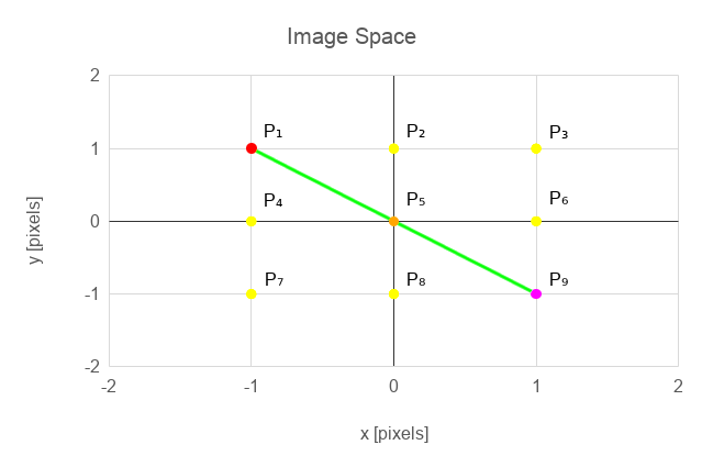
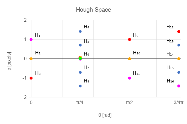
Figure 3.a, 3.b Points P1, P2 and Line L1 in image space (left) and hough space (right)
What we can notice here is that we got rid of the coordinates and the transformation and inverse transformation remove the need to calculate anything but still give us the ability to use the efficiency of the Randomized Hough Transform.
So, H1,...,H16 represents lines in image space. We not just got rid of coordinate system, but the information is compressed without (unintentionally) loosing any details. Moreover, we can go further. As I mentioned earlier, normally when Hough transform is applied in computer vision, to achieve any sort of invariance (position, rotation, scale) additional parameters are added to the parameters space, but hugely compromising performance. We can achieve similar things just by adding additional set of transformations on top of previous one. We can combine terms representing different properties of an object from any image/parameter spaces, so we can be as general or specific as we want to be, and we can do it very effectively. A single term can represent a very general object and if we use it together with a term that has any specific information (location, rotation, scale) that led to the recognition of general term, than we have a term representing a general object but also with some specific properties.
A subset of transformation statements that illustrate how to build from simple features more complex and how to add or remove specificity:
- H1, H2, H3 → H⇒
H1, H2, H3 are specific horizontal lines, whereas H⇒ represent any of them. - H4, H5, H6, H7, H8 → H⇗
Same but with a slope of 45°. - H9, H10, H11 → H⇑
Vertical lines. - H12, H13, H14, H15, H16 → H⇖
Lines with a slope of 135°. - H⇒, H⇑ → H+
Perpendicular lines composed from horizontal and vertical line(s). - H⇗, H⇖ → Hx
Same, but rotated by 45°. - H+, Hx → HL
Perpendicular rotation invariant lines. - P1', P9', H6 → L1
A line segment with an exact location, P1' and P9' are end stop points, that are different from P1 and P9 which are just ordinary edge points. Line does not continue beyond them, so those points need to be specifically detected. Also a line segment without an exact location, with length and/or rotation invariance can be similarly constructed to use it in a more general way e.g. L1, L2... → Linv.
Another example could be to do Hough or similar transformations recursively. E.g. if we do a line Hough transform on a circle centered at the beginning of a coordinate system, we get a set of sinusoids in parameter space enveloped by two distinct horizontal lines ρ and -ρ. Applying the same transformation again, we get two points that represent that envelop in the previous parameter space, which represent a circle in image space. What this all resemble is how simple, complex and hyper-complex cells hierarchically represents objects as its been described in many research studies of neurobiologist. In those examples we used equation (2) from a line Hough transform, but in general we can use any equation, or even transformations that doesn't have any analytical form.
Because of discretization of the image space some question still need to be solved. How to effectively apply transformations on image space(s)? Using small partially overlapped regions, or using a global log polar coordinates system, a combination of those or something entirely different? In Cartesian coordinate system we highly compromising effectiveness and resolution
Now, one more question still remains, how to effectively implement all of this?
An efficient system running Symbolic Hough Transform
While NARS is very well designed to handle such a task, in my opinion, currently other system might easily outperform it in terms of speed. To try out the algorithm, I decided to create a new simplistic system, and mainly target performance, So I took NARS and tried to simplify to the extent just to be able to handle this single task and create a control mechanism that would target performance. Information will be still represented in a similar but simplistic way to NARS. Here nodes will represent terms and edges relations between terms. Also, ability to learn will remain, but might be different from the original NARS design. The control mechanism is inspired by Petri net. Petri net is a type of Discrete event dynamic system, which is a tool to model various concurrency and synchronization problems in distributed and parallel processing systems. Also some features of the system will be inspired by biological neural systems although those will not try to be accurate but its usage will be justified by its helpfulness in this particular context. It has some resemblance with neural networks, but the network is dynamic (new connections are added or removed on the fly) and its calculations are more efficient (it is not preformed in a global level, but just those parts where it is necessary). All in all – whatever works, no matter how bizarre it seems to be, is equally good (in my opinion) if we get the expected results.
Event Network
(to be refined)

Figure 4 Basic elements of the event network


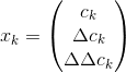
Let's have a system with a set of nodes and edges, where nodes represent terms and edges relations between those terms. A node can be activated in a similar way than in Petri Nets, but there will be differences. Markings (in Petri Nets "tokens", here "potential" ui) will be held by edges, not nodes (places in Petri Nets) and they will be a real number from < -1., 1.> and will be a subject to a time degradation. There will be no special elements like transitions, here the firing will be directly on nodes and the process of firing will be called event which will have the same name as the node itself. The event will trigger computation - on every outgoing connections, ui will be updated, and checked whether it activates a node. When a node fires, it produces a potential with a value 1.0 to all its outgoing connections, but also looses its potential in all incoming connections (except on nodes with graded potential). The value of potential of all outgoing connection for the node that has been fired will be updated. The real value of the tokens on the connection will be 1.0 * wi added to existing value degraded by time (here Δt means time interval since last update of ui), and the sum of weight for all connection for a particular node will be also 1.0 or -1.0 (for wi < 0, to be able to block activation). The weights are not constant but changing depending on its usage. Also new connection can be made or weak one deleted. New connection will be made in a bit similar fashion than it is in NARS, although the rules will be not so strict. In neurobiology there is a theory that says "what fires together wires together.", so new connection will be made based on time and space proximity of nodes. Time proximity means, if events, representing firing nodes will often fire together (within small interval Δt) and they are spatially close – a connection will be made (weight of other connection related those nodes will be adjusted to keep sum of weight = 1.0). Firing of a node will occur when the sum of markings multiplied by the weights will be higher than a certain global) threshold. This marking can be also summed up during time, when multiple firing occurs on the same connection but the node, where this connection is entering, was not activated yet.. Some of input connection can be negations to block certain events and prevent further processing.
Action potential vs Graded potential: Action potential is a source of single event. Graded potential is a periodical generator of events, which frequency depends on the value of a grade – usually used for sensors.

Figure 5 A very simplified version of our line detector using Event Network emulating Randomized Hough Transform
Overall architecture of Visual Perception using Event Network
(to be refined)

Figure 6 Overall architecture of visual processing
Comparison to other systems
(to be refined)
Deep Neural networks/Convolutional Neural Networks, SIFT and similar, Classical Hough Although neural networks are widely used for image categorization, they have a lots of problems:
- Computes always everything (NN)
- loosing information (CNN)
- no relationship between detected local features (most of the techniques or algorithm)
- does not understand context (NN)
- after design, the structure remains fixed, after training weights remain fixed (NN)
Possible applications
(to be refined)
This system has a potential to be used not just for Visual perception or other kind of perceptions, perhaps NLP but also as a part of a universal problem solver. Mapping a problem to a different parameter space with a combination of effective techniques to find required solution with the ability to learn could be a powerful tool for various real world applications. Moreover it is simple enough to be easily implemented.
(to be extended)
1 Ramps-Antiramps and the red queen - An early genetic algorithm (From Charles Ofria )
2 Perception from an AGI Perspective (By Pei Wang and Patrick Hammer)
[Proceedings of AGI-18, Prague, Czech, August 2018]
Perception in AGI should be subjective, active, and unified with other cognitive processes
Speech Recognition using NARS
Written by Pavol Durisek- Details
-
Category: Articles
-
Published: 09 January 2014
-
Hits: 9540
Introduction
NARS takes a single major technique to carry out various cognitive functions and to solve various problems. This technique enables to model any aspect of an intelligent system – perception, cognition, reasoning, consciousness … in a unified way.
Dr. Pei Wang already published many papers about the NARS capabilities, most notably, the one about problem solving case-by-case manner without using a known algorithm.
In this article I would like to demonstrate that NARS can be used as well for other task without using a special module, technique or tool attached to a system.
NARS is ideal for dealing with perception for many reason. As it with the problem solving, when there is an absence of an exact algorithm to solve the (even a very simple) problem, in perception, problems occur with information ambiguity (inverse optics problem), its correctness (source of information might infer with other sources) and completeness.
So some information might be lost, some are not accurate, and even though having everything right, the interpretation and importance of any perceived information is system dependent.
The following diagram shows the common framework for state-of-the-art ASR (Automatic Speech Recognition) systems, which has been fairly stable for about two decades now and a proposed ASR using NARS.


Figure 1.a, 1.b Speech recognition conventional, and using NARS
A transformation of a short-term power spectral estimate is computed every 10ms, and then is used as an observation vector for Gaussian-mixture-based HMMs that have been trained on as much data as possible, augmented by prior probabilities for word sequences generated by smoothed counts from many examples.
Many feature extraction methods, that have been used for automatic speech recognition (ASR) have either been inspired by analogy to biological mechanisms, or at least have similar functional properties to biological or psycho-acoustic properties for humans or other mammals.
The most common features used today in ASR systems are MFCC (Mel-scale Frequency Cepstral Coefficient). For non-speech audio classification purposes, or to improve accuracy, also other audio features are commonly used or their combination. The following chapter shows simple steps how to obtain MFCC from audio signal.
Calculating (MFCC) audio features
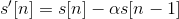
Input analog signal x(t) is converted to a discrete valued discrete time signal s[n] at a sample rate f.
Bellow, some simple steps shows, how to obtain MFCC (Mel Frequency Cepstral Coefficients) from this converted audio signal1,2.
Step 1: Pre–emphasis
To compensate the high-frequency part that was suppressed during the sound production mechanism of humans and also to improve signal-to-noise ratio, audio signal are passed through the high pass filter.
Step 2: Framing
The signal is then framed into small chunks with some overlap. Usually the frame width is 25ms with an overlap 10ms.
Step 3: Hamming windowing
In order to apply spectral analysis to a frame, it has to be multiplied with a window, to keep the continuity of the first and the last point and avoiding “spectral leakage”.

Hamming window is defined as:
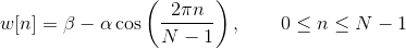
, where N represents the width, in samples, of a discrete-time.

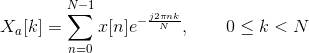
Step 4: Fourier transform of the signal
FFT is performed to obtain the magnitude frequency response of each frame. Spectral analysis shows that different timbres in speech signals corresponds to different energy distribution over frequencies.
Step 5: Mel Filter Bank Processing
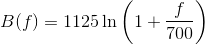
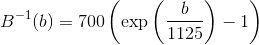
Non-linear frequency scale is used, which approximates the behaviour of the auditory system. The mel scale is a perceptual scale of pitches judged by listeners to be equal in distance from one another.
The mel-scale B and its inverse B-1 can be given by Eq (different authors use different formulas):
We define a filter bank with M filters, where filter m is triangular filter given by:
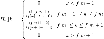
Such filters compute the average spectrum around each center frequency with increasing bandwidths.
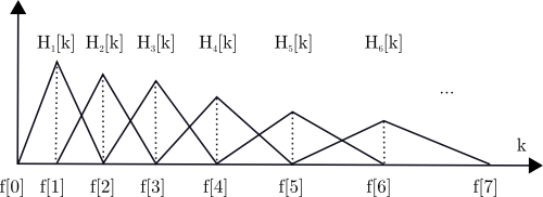
Figure 2 Triangular mel-scale filter banks (normalized)
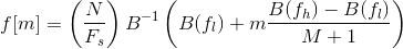
Let’s define fl and fh to be the lowest and highest frequencies of the filter bank in Hz, Fs the sampling frequency in Hz, M the number of filters, and N the size of the FFT. The boundary points f[m] are uniformly spaced in the mel-scale:
Step 6: Discrete Cosine Transform
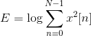
We then compute the log-energy at the output of each filter as
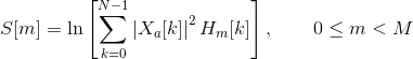
The mel frequency cepstrum is then the discrete cosine transform of the M filter outputs:
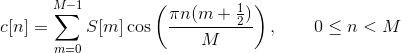
Discrete cosine transform decorrelates the features (improves statistical properties by removing correlations between the features).
Step 6: Feature vector
The energy within a frame is also an important feature that can be easily obtained. Hence we usually add the log energy as the 13rd feature to MFCC. If necessary, we can add some other features at this step, including pitch, zero cross rate, high-order spectrum momentum, and so on.
It is also advantageous to have the time derivatives of (energy+MFCC) as new features as velocity and acceleration coefficients (which are simply the 1st and 2nd time derivative of cepstral coefficients respectively).
Together with delta (velocity) and delta-delta (acceleration) coefficients, represents the audio feature vector used in conventional ASR..
Representing audio features in Narsese
All the stages so far, shared common parts in conventional and ASR using NARS. Conventional ASR uses HMM (Hidden Markov Model) in next stages which incorporates acoustic and language models.
While numerical representation of feature facilitate processing and statistical analysis in conventional ASR (real numbers, fixed information structure), which is appropriate given its statistical nature, in NARS however, features needed to be converted to Narsese. Two questions arise here:
- How to represent numerical values?
- How to represent temporariness of attributes?
It would be possible to use other modules attached to NARS and do numerical calculations, but this is what tried to be avoided from the beginning.
Representing numerical values
Usually, there is no need to represent exact numerical values in perception unless we want to represent numbers itself. In perception the accuracy of recognition is not necesarilly proportional to accuracy of received information. If we were a green-tinted glasses or replace our white light bulb with a green one, we will notice the tint, but we still identify bananas as yellow, paper as white, walls as brown (or whatever), and so forth. So the wavelengths of light does not correspond to colours we experience (or we want the system to experience) no matter how accurately we perceive it. The same information might be seen differently dependent on certain conditions and the system previous experience.
To be able to uniquely identify and classify certain information or object, we need to choose the right features. While some of them should be similaritive (invariant to certain properties) to classify as the same category of objects, others, should be distinctive, to uniquely identify object within the same class. There is no need an exhaustive list of all features we can gather nor concentrating to get it as precisely as we can (anyway we would not get it right - as it implies from the mentioned example above). So not the number of coefficients and its accuracy, but rather the character of features, its adaptive choice based on current conditions and the amount of experience and its variety the system has what matters the most.
Representing temporal attributes
The validity of information (statements - in NARS terminology) might be time dependent. In Pei Wang's NARS design, there are tree mechanism to deal with temporal statements3.
- Relative representation. Some compound terms (implication, equivalence, and conjunction) may have temporal order specified among its components.
- Numerical representation. A sentence has a time stamp to indicate its "creation time", plus an optional "tense" or its truth-value, with respect to this time.
- Explicit representation. When the above representations cannot satisfy the accuracy requirement when temporal information is needed, it is always possible to introduce terms to explicitly represent an event or a temporal relation.
The explicit representation is the most basic one, since it doesn’t requires to implement temporal inference rules, but time and events are expressed as terms. The first approach is not implemented yet in the library presented on this site, but a limited version of second - numerical representation of temporal statements is implemented with following properties:
- The temporal statement is indicated by a tense (currently just "|⇒", which represents a present tense by Wang's NAL) and a time stamp is attached to it to represent the creation time.
- Every temporal statement keeps its truth value for a short period of time after which the statement is discarded from the system.
- It is still a way to remember a whole history of temporal statements, by (periodically) assigning the value to a new term before it gets discarded.
- Any statement derived from a temporal statement is also temporal.
The advantage of temporal statements to represent features in perception this way is, that system does not have to update the states of all those features, whenever their change. Remember, that in conventional ASR, the whole feature vector are feeded into system by every frame, which also limits the amount of features used in the system. However in NARS by the next frame, temporal features from previous frame are already deprecated, so the actual list of used features might differ from frame to from, and it is not limited either by number or type.
Possible implementation
This chapter shows a working demonstration, how such a system could be implemented. For simplicity, it will be explained just on recognising vowels, given, this is one of the simplest task in speech recognition process.
This demonstration uses NARS library available on this website together with FFTW library which handles calculation of audio features from the input signal. The test program was able to process in real-time requiring very little computer resources.
The following charts are based on this audio recording of words with General American English vowels illustrated on Table 1.
| b__d | IPA | b__d | IPA | ||
|---|---|---|---|---|---|
| 1 | bead | iː | 9 | bode | oʊ |
| 2 | bid | ɪ | 10 | booed | uː |
| 3 | bayed | eɪ | 11 | bud | ʌ |
| 4 | bed | ɛ | 12 | bird | ɜː |
| 5 | bad | æ | 13 | bide | aɪ |
| 6 | bod(y) | ɑː | 14 | bowed | aʊ |
| 7 | bawd | ɔː | 15 | Boyd | ɔɪ |
| 8 | budd(hist) | ʊ |
A certain threshold of log energy of a frame can be used to indicate of the beginning and the end of a word thus the processing.
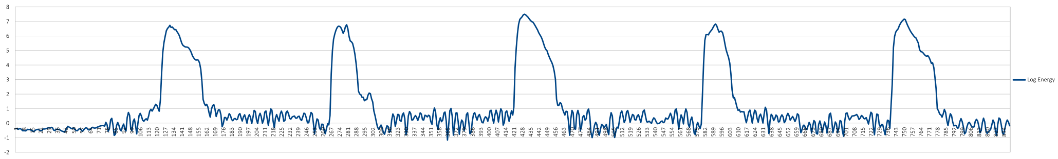
Figure 2 Log Energy of each frame (x-frame number, y-log energy of a frame)
On Figure 3, one could notice, that the energy level of bands (for clarity is shown just the first four), represented by cepstral coefficients within a vowel are quite constant. One possible solution to recognise them could be to either measure the value of each cepstral coefficient (which is tried to be avoid, as it was mention in the chapter about the numerical representation) or measuring their relative order to each other. But that could be also misleading, since not the actual values but rather the positions of frequency bands with high (and low) energy what matters. Depending on the speaker, this might also slightly change, so having more Narsese rules for every vowel could be very handy. Moreover, we might get also information about the speaker (high or low pitch voice, gender etc.).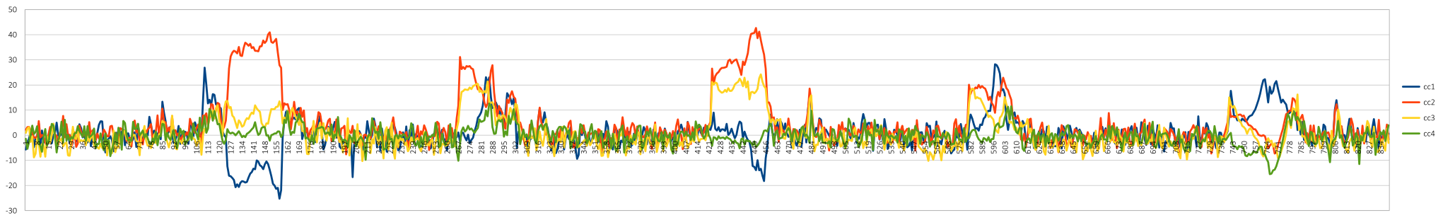
Figure 3 Vowels and their mel scale cepstral coefficients
Figure 4 is the same recording showing the values of coefficients, but from different perspective. Here, the time is static (in vowels the cepstral coefficient are not time dependant), and showing the value of cepstral coefficients for different vowels (we would like to differentiate one vowel from others). This chart clearly show, that just by featuring maxima and minima, we could uniquely identify vowels.
As for consonants, we would need to take to account the time dependant coefficients (velocity and acceleration).
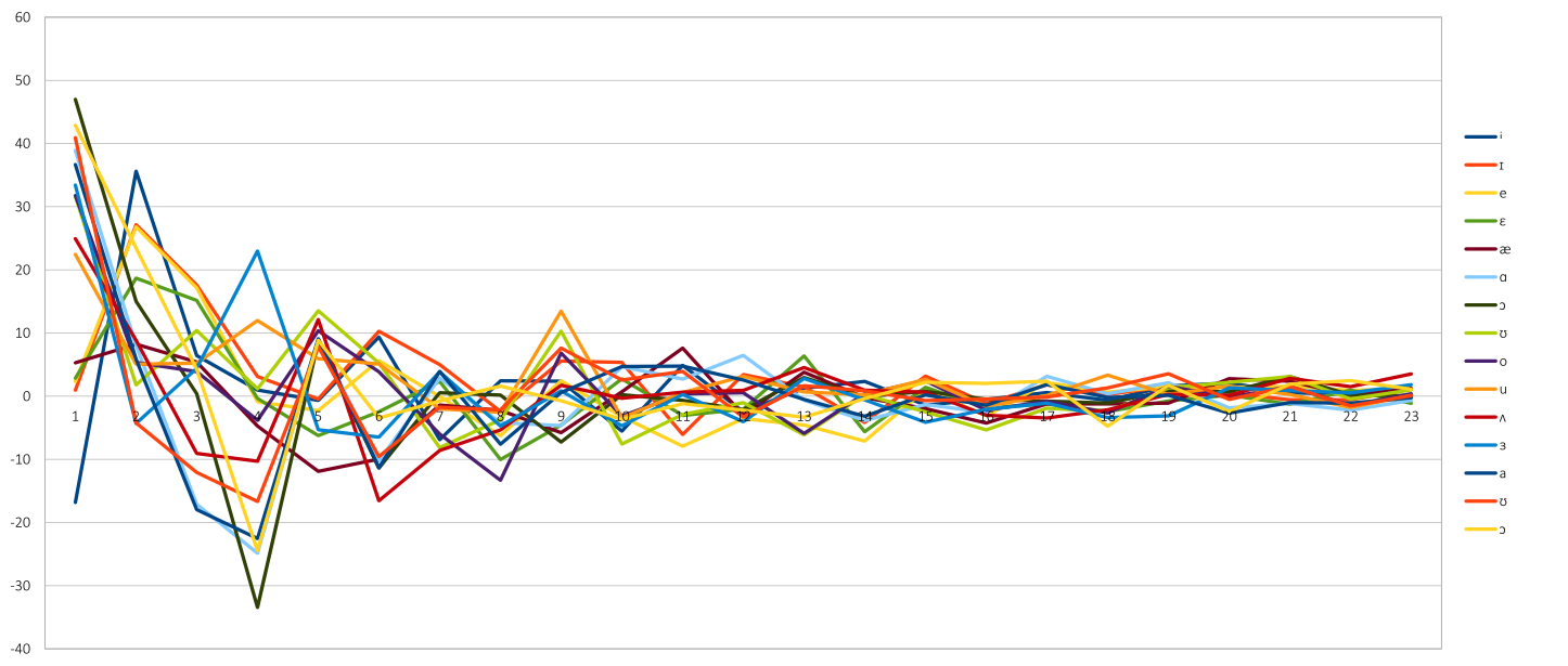
Figure 4 Vowels and their mel scale cepstral coefficients (x-cepstral coefficient, y-log energy)
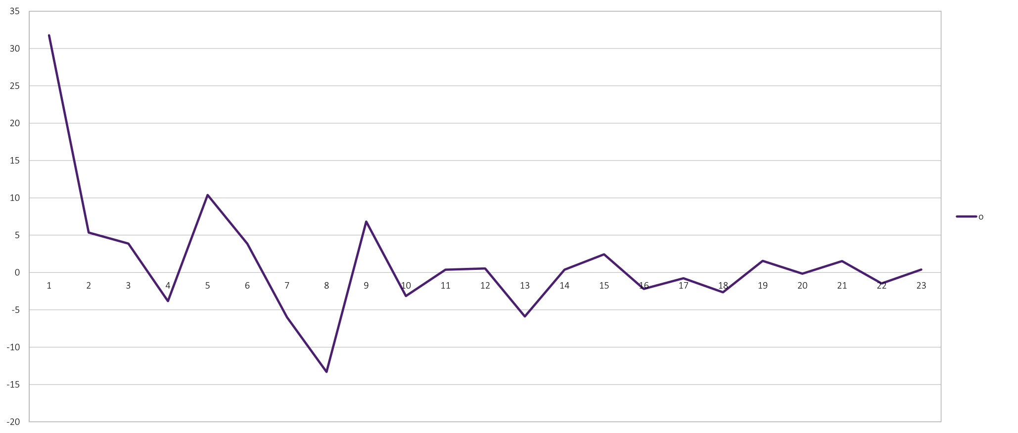
Figure 5 Vowel "o" and its mel scale cepstral coefficients (taken from Figure 4)
|
1
|
((∧, (cc1 → [max]), (cc4 → [min]), (cc5 → [max]), (cc8 → [min]), (cc9 → [max]), (cc13 → [min])) ⇒ ({o} → current_sound)).
|
Code 1 Vowel "o" and its features in Narsese
Code 1 shows a possible representation of vowel 'o' in Narsese. Every vowel could have multiple rules attached to it and also rules to recognise other attributes of speech, like pitch, intonations etc..
|
1
2
3
4
5
6
7
8
9
10
11
12
|
((∧, (cc1 → [min]), (cc2 → [max]), (cc5 → [min]), (cc6 → [max]), (cc7 → [min]), (cc8 → [max]), (cc10 → [min]), (cc11 → [max])) ⇒ ({i} → current_sound)). ((∧, (cc1 → [min]), (cc2 → [max]), (cc5 → [min]), (cc6 → [max]), (cc8 → [min]), (cc9 → [max]), (cc11 → [min]), (cc12 → [max]), (cc14 → [min])) ⇒ ({ɪ} → current_sound)). ((∧, (cc1 → [min]), (cc2 → [max]), (cc5 → [min]), (cc6 → [max]), (cc8 → [min]), (cc9 → [max]), (cc14 → [min])) ⇒ ({e} → current_sound)). ((∧, (cc1 → [min]), (cc2 → [max]), (cc5 → [min]), (cc7 → [max]), (cc8 → [min]), (cc10 → [max]), (cc11 → [min]), (cc13 → [max])) ⇒ ({ɛ} → current_sound)). ((∧, (cc2 → [max]), (cc5 → [min]), (cc11 → [max]), (cc12 → [min])) ⇒ ({æ} → current_sound)). ((∧, (cc1 → [max]), (cc4 → [min]), (cc5 → [max]), (cc6 → [min]), (cc7 → [max]), (cc9 → [min]), (cc12 → [max])) ⇒ ({ɑ} → current_sound)). ((∧, (cc1 → [max]), (cc4 → [min]), (cc5 → [max]), (cc6 → [min]), (cc7 → [max]), (cc9 → [min])) ⇒ ({ɔ} → current_sound)). ((∧, (cc1 → [max]), (cc2 → [min]), (cc3 → [max]), (cc4 → [min]), (cc5 → [max]), (cc7 → [min]), (cc9 → [max]), (cc10 → [min]), (cc12 → [max]), (cc13 → [min])) ⇒ ({ʊ} → current_sound)). ((∧, (cc1 → [max]), (cc4 → [min]), (cc5 → [max]), (cc8 → [min]), (cc9 → [max]), (cc13 → [min])) ⇒ ({o} → current_sound)). ((∧, (cc1 → [max]), (cc2 → [min]), (cc4 → [max]), (cc8 → [min]), (cc9 → [max]), (cc10 → [min])) ⇒ ({u} → current_sound)). ((∧, (cc1 → [max]), (cc4 → [min]), (cc5 → [max]), (cc6 → [min])) ⇒ ({ʌ} → current_sound)). ((∧, (cc1 → [max]), (cc2 → [min]), (cc4 → [max]), (cc6 → [min]), (cc7 → [max]), (cc8 → [min])) ⇒ ({ɜ} → current_sound)). |
Code 2 Representing all the vowels from Table 1 in Narsese
|
1
2
3
4
5
6
|
|⇒ (cc1 → [max]). <1, 0.9> |⇒ (cc4 → [min]). <1, 0.9> |⇒ (cc5 → [max]). <1, 0.9> |⇒ (cc8 → [min]). <1, 0.9> |⇒ (cc9 → [max]). <1, 0.9> |⇒ (cc13 → [min]). <1, 0.9> |
Code 3 Vowel "o" represented in Narsese
|
1
2
3
4
5
6
|
|⇒ (cc1 → [max]). |⇒ (cc4 → [min]). |⇒ (cc5 → [max]). |⇒ (cc8 → [min]). |⇒ (cc9 → [max]). |⇒ (cc13 → [min]). |
Code 4 Same as in Code 3, but with default truth values
|
7
|
(? → current_sound)? |
Code 5 an example question asked after features are entered to the system by every frame.
Code 2 representing a knowledge base needed for speech processing, and which is already stored in the system, and Code 3 or Code 4 and Code 5 is an example, how features might be converted to Narsese and sent to the system by every frame.
So the basic concept is, that system would contain knowledge about the language (similarly to acoustic and language model in conventional ASR) in Narsese and features would enter to the system (also in Narsese) together with some questions and/or goals. Than system would provide some answers and perhaps actions. A full featured ASR would require much more sophisticated rules than it was shown previously and also there arise a question, how to automatically build such a knowledge base.
But the advantage could be huge. The knowledge is shared in the whole system, so also information coming from other type of sensory sources could be used. The same system could be used also for visual perception or for controlling sensory motors. Also, system could use active sensors to better adapt to current conditions and surrounding environment.
1. Xuedong Huang, Alex Acero, Hsiao-Wuen Hon (May 5, 2001), Spoken Language Processing: A Guide to Theory, Algorithm and System Development
2. Roger Jang (張智星), Audio Signal Processing and Recognition
3. Pei Wang (May 6, 2013), Non-Axiomatic Logic: A Model of Intelligent Reasoning